Tips for Excel, Word, PowerPoint and Other Applications

Advanced Applications of SUMPRODUCT (part 2)

Why It Matters To You

The more I use the advanced capabilities of SUMPRODUCT, the more I like it. In this tutorial, we'll walk through how to use part of a cell's contents as the conditional test.

If you can use a part of a cell's contents as a conditional test, then how you set up your data in the first place is important. The example here is actually a derivative of something I set up at my work.

How to ...

You can use the example file, sumproduct_advanced2.xls, to follow along and see examples.

In this example, I have 3 business units, called Unit1, Unit2, and Unit3. Each one has an HR and an IT department, and we're trying to summarize budgets for the next year. Advanced SUMPRODUCT can help you summarize budgets for any of the business units or for any of the departments. In my case at work, I mapped each cost center to a business unit using the format: [company]-[department]. I did this because I was dealing with multiple business units that had the same departments (e.g., IT and HR) and wanted to be able to segregate Unit1 from Unit2, but also wanted to aggregate across common departments if needed.

In this example, let's assume that I'm doing some budget planning for various departments across multiple business units. The data, rolled up at a department level, might look like this.

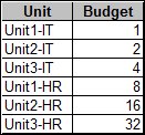
We're going to use our trusty SUMPRODUCT function to do two things: summarize budget for Unit2 and then for the IT departments. You'll notice that I can segregate all of the Unit2 values if I can parse the left 5 characters of the Unit and I can segregate all of the IT values if I can parse the right 2 values of the Unit. We can do this with our LEFT and RIGHT functions.

So, if you followed Advanced SUMPRODUCT (Part 1), you'll remember that all I have to do is to write a logical test as one of my arrays. The final formula to summarize budget for Unit2 might look like this:

SUMPRODUCT(--(LEFT($B$5:$B$10,5)=B14),$C$5:$C$10)

The array defined as "--(LEFT($B$5:$B$10,5)=B14)" tests the leftmost 5 characters to see if it's equal to B14 (aka "Unit2) and then coverts them to 1's and 0's. When combined with the actual values, it only includes the Unit2 values.

A RIGHT formula works in a similar fashion. We can use this to summarize budget for IT vs HR like this:

SUMPRODUCT(--(RIGHT($B$5:$B$10,2)=B18),$C$5:$C$10)

So What?

This is powerful. A pivot table can't do this. You could do this if you parsed the Units column into separate columns, but sometimes that can be messy. This is a way to execute the summary in one easy formula. Not only can you specify what summary values you want, but the formula is dynamic and can be easily copied and pasted.

Notes

Last updated	2/28/08
Application Version	Excel 2003
Author	Michael Kan
Pre-requisites	Basic SUMPRODUCT Advanced SUMPRODUCT (Part 1) Text Parsing in Excel: LEFT, MID, RIGHT Introduction to Logical Statements and Logical Math
Related Tips	Advanced SUMPRODUCT (Part 3) Advanced SUMPRODUCT (Part 4)