Tips for Excel, Word, PowerPoint and Other Applications

Advanced Applications of SUMPRODUCT (part 1)

Why It Matters To You

If SUMPRODUCT is one of the handful of must know functions, advanced SUMPRODUCT is even more useful. How often do you only need to summarize by a single criteria? You never need to know just sales by region, it's always sales by product by rep by region. Or, if you're evaluating home expenses, it's gas expenses by month.

It gets better. SUMPRODUCT supports a wide range of conditional summation such as part of a cell's contents (part 2), only odd numbers (part 3), or only for values where an associated field is blank (part 4). While you might not be particularly interested in any of these particular examples, it does highlight the flexibility of SUMPRODUCT.

So why not use a Pivot Table? In my opinion, Advanced SUMPRODUCT delivers better summary capabilities than a pivot table and allows you to control the layout and usage of the output better than a pivot table. SUMPRODUCTs also update dynamically, unlike pivot tables which must be refreshed, so the outputs can be used in models quite nicely.

How to ...

You can use the example file, sumproduct_advanced1.xls, to follow along and try out the examples.

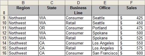
For our example data set, we're going to use the table below, which shows Sales by Region, State, Business Line, and Office? What can we use to determine, say Sales for just the Northwest region or what about just the Commerical line in the Northwest Region?

Potential Alternatives

SUMIF could be an option, if we only have a single filter criteria, or an ARRAY statement, which always seems to throw people into seizures, or even a Pivot Table, which can get messy, especially if you're only interested in a small portion of the data.

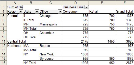
Let's start off by taking a look at what a Pivot Table would generate. It does a fair job at summarizing the data, but the layout is ugly and if your data changes, let's say you add another month to the data set, the size and dimensions of your resulting pivot table changes. This might break any formulas linked to your pivot table data. Also, the more complex your pivot table summary, the dirtier your pivot table will be.

I won't talk much about ARRAY formulas, but SUMIFs are really limited to a single criteria (e.g., Commercial OR California OR Northwest) but not a combination of them.

So let's get to the subject of this Tip, which is SUMPRODUCT. If you need a refresher, click over to the article on Basic SUMPRODUCT.

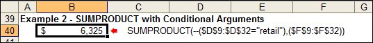
Typically, the SUMPRODUCT formula is written as a series of arrays, the respective (e.g., first, second, … nth) values of which will be multiplied together, then the results will all be summed. Let's write a SUMPRODUCT function to calculate the Sales, but only for Retail.

If you used the function wizard to build your SUMPRODUCT formula, you'd get something like this:

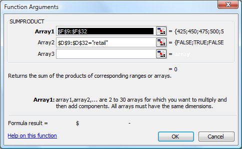
Array 1 contains all of my Sales values

Array 2 is looking only for the values which = "Retail"

Note: Notice how all of the values in Array 2 are reported as TRUE or FALSE? If you go back to our example data set, you'll see the first value in Column D is Consumer, resulting in FALSE and the second value is Retail, which results in a TRUE value. (Introduction to Logical Statements and Logical Math )

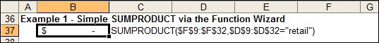
Unfortunately, the function doesn't work. It returned a value of 0. The reason for this is that Excel doesn't know how to handle the series of TRUE and FALSE values.

So we're going to adjust our formula by adding a ' -- ' (double unary) in front of all of the conditional statements to transform the TRUE and FALSE values into 0's and 1's, which now yields the results we want.

To be perfectly honest, I don't really know why this works, only that it does. It's probably easier to show you what happens by way of some examples and screenshots from the Formula Bar. Go the cell B40 in the example file, highlight the indicated sections of the forumula, and then hit F9. F9 will show you the calculated value of any piece of a formula. It's very handy for troubleshooting your formulas. Just remember to hit ESC so that your values don't stay hard coded.

If I only highlight the conditional statement and hit F9, ...

... it returns TRUE or FALSE results, which I know from my previous experiment won't work.

However, if I highlight the parentheses and the double unary, and hit F9, ...

... all of my TRUE and FALSE results are transformed into 1's and 0's, which is very useful.

Still on the bus? Now let's figure out Sales for Retail, but only for the Northwest Region.

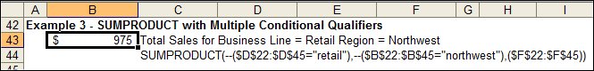
If you followed the previous example, you'll now realize that the SUMPRODUCT is testing each cell in the Business Line array and returning a value of 1 where Business Line = "retail" and testing each cell in the Region array and returning a value of 1 where Region = "northwest". The resulting math results in a combined value of 1 ONLY where Business Line = "retail" AND Region = "northwest". Every other combination returns a value of 0. Carry this one step further and you'll see that this, combined with your sales figures, totals only what you wanted to see and nothing else.

So What?

In my opinion, this is a much cleaner way of getting to targeted summary figures than a Pivot Table. Not only can you specify what summary values you want, but the formula is dynamic and can be easily copied and pasted. Also, you might have also realized that instead of using hard coded values like "northwest" and "retail", you could replace these with drop down boxes or other methods of generating inputs. We'll cover more on this in a separate article. Enjoy.

Notes

Last updated	8/21/08
Application Version	Excel 2003
Author	Michael Kan
Pre-requisites	Basic SUMPRODUCT
Related Tips	Introduction to Logical Statements and Logical Math Advanced SUMPRODUCT (Part 2) Advanced SUMPRODUCT (Part 3) Advanced SUMPRODUCT (Part 4)