
Tips for Excel, Word, PowerPoint and Other Applications
Introduction to Basic Pivot Tables in Excel
Why It Matters To You
Pivot tables are one of the easiest analytical tools available to quickly summarize a large amount of data. They have their limitations, but as long as you understand where they are powerful and where they are limited, you should be good to go. I've written up a quick step by step of how to including a sample data set on which you can try out the Pivot table functionality.
Pivot tables are useful anytime you want to quickly summarize data (cross tabs). They a great for quickly creating a table of summary results and better yet, let you double-click to see all the detail underlying any specific value. The drop downs at the X, Y, and page level let you quickly filter data for very specific looks at your data.
Notes of Caution
- Pivot tables are only as good as the underlying source data, meaning that if you have 10 different spelling of the same supplier, location, or employee, it will report each as a separate item.
- Pivot tables are semi-dynamic, meaning that you must mnaually refresh data to update numbers.
- The structure of a pivot tables is dynamic. If you change the items on your x and y axes, your pivot table will change accordingly, upon refresh, which are a good thing and a bad thing. This also means that it's hard to link to a pivot table for source data, because the target cell may change.
- Pivot tables will bloat the size of your file. Try it out. Grab a big data set, check the file size before and after making a pivot table and you'll see that your file size can increase by 100-200%.
- Because your pivot table is semi-dynamic, you are forced to copy and paste values as values if you want to use the results in a model, which means it's a pain to update your model if the underlying data set changes regularly.
Overcoming Some of the Limitations of Pivot Tables
- A little bit of data cleaning prior to running your pivot table can pay off significantly. Use Pivot tables and VLOOKUPs to collapse your raw data into something more useable (e.g., collapsing the 10 ship to locations for Home Office (HOMEOFF87 into the general location 'HOMEOFFICE').
- If you know what cross tabs you need and the number is small, CONCATENATE, SUMIF, and SUMPRODUCT can create the same functionality.
- Use of CONCATENATE and SUMIF, or SUMPRODUCT also allows you to 1) control the size and shape of your cross tab summary, 2) dynamically reflect changes in your underlying data, and 3) use the summarized data for downstream modelling.
How To ...
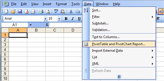
The following discussion references the Excel file pivot_basic.xls, so download that first and let's go. First, go Main Menu:File:Pivot Table (ALT, D, P) to launch the Pivot Table Wizard. You can do this before or after selecting a data range.
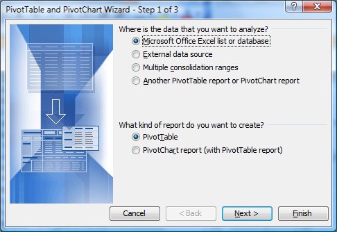
The Pivot Table Wizard (hereafter referred to as the 'Wizard') will walk you through a simple 3-step process. For the rest of this Tip, we'll use the data provided in the tab named 'Invoice Sample', which is an extract of an 2,000+ line invoice file. Lines have been cut to protect the innocent, and the pricinples are the same in any case. In fact, you can use the same data set to practice building your own pivot table.
For the source of the data, select Microsoft Excel list or database. Click 'Next'.
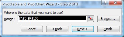
The Wizard will now ask you what range you want to use (Step 2 of 3). Click on the tab 'Invoice Sample, highlight everything from the column headers to the bottom right hand corner data cell. Column headers are critical since those will create the X, Y and page tabs. Click 'Next'.
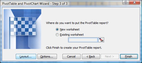
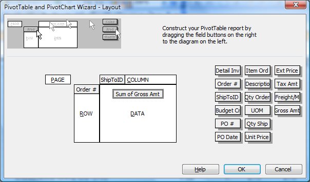
Step 3 of 3 asks you how you want your pivot table to look and where you want to put it. Select 'Layout'.
The Layout wizard is a drag and drop interface that lets you select how you want to summarize data at the page, X, and Y level. If you drag a data header into the Row area, your pivot table will have all of the unique values displayed on the vertical. This abilty, by itself, is quite useful.
Drag the box labeled PO# into the row area and drag ShipToID into the column area. Next, drag Gross Amt into the data area. You should see the label convert to either Sum of Gross Amt or Count of Gross Amt.
Let's stop here and review what's going to happen. We are asking Excel to display all of the unique PO# values on the vertical and all of the unique ShipToID values on the horizontal, then for each intersection, calculate the total Gross Amt.
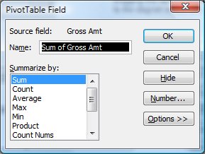
If you want to change the type of summary performed, double-click Sum of Gross Amt and you should see the following box open up. This will let you customize the type of summary operation as well as the number format and some other stuff (e.g., Options >>)
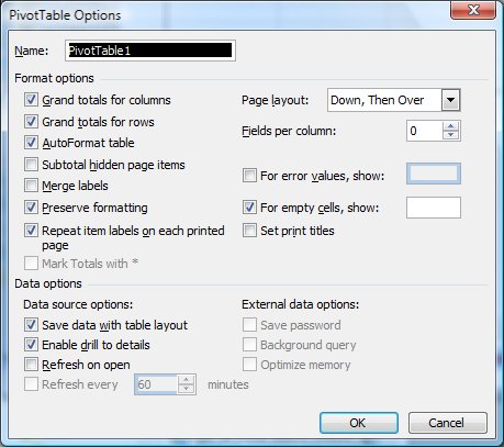
Once you get back to the main Step 3 of 3 window, you can also click Options, which will launch the following window. This provides some other formating and layout options. I suggest that you just play around with some of these to see what they do.
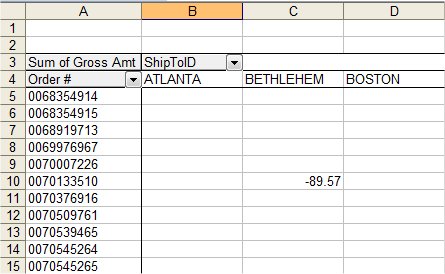
Click OK to return to the Step 3 of 3 page, click Finish, and it will create a new sheet with your pivot table, which should look like this. You'll notice that your data fields are presented, with drop down boxes, along the vertical and horitzontal axes. Your summary criteria is shown in the upper left hand corner.
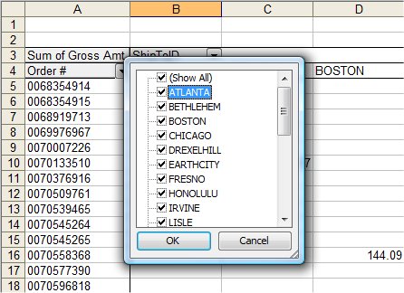
Here's where Pivot Tables are very powerful. Click on the ShipToID dropdown and you'll see all of your locations with a check next to them. You can uncheck any of them to selectively exclude them from the analysis. You can do the same for PO# or anything in the Page view.
Now, click on ShipToID and drag it onto the vertical axis ...
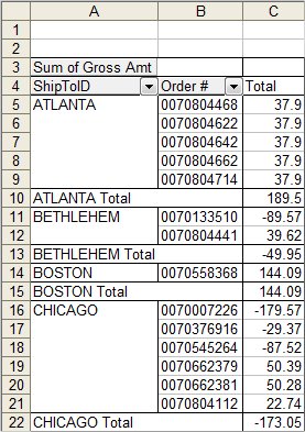
... and your Pivot Table will reorganize. You can also drag data labels into the Page View. Now double-click any summary value in a pivot table and Excel will open up a new sheet showing you all of the PO lines that contributed to that value.
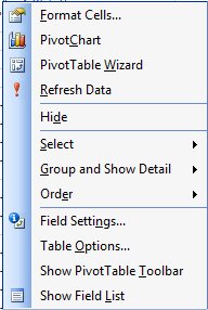
Lastly, if you ever need to refresh the data in your Pivot Table (added new data, changed data, etc), just right-click in the body of your Pivot Table, you will see the option bar below, then select Refresh Data. You can also select Wizard if you want to go back and adjust formating options or the layout of your table.
That's it. Play around a bit and see for yourself what Pivot Tables can do. When you're ready for a challenge, head over to the 15-Second Pivot Table article to build proficiency.
Notes
| Last updated | 9/2/07 |
| Application Version | Excel 2003 |
| Author | Michael Kan |
| Pre-requisites | None |
| Related Tips |