
Tips for Excel, Word, PowerPoint and Other Applications
Highlighting the Top N Values
Why It Matters to You
We talked recently about several ranking functions: RANK, LARGE, and SMALL. These can also be used with Conditional Formatting and user controlled ranking criteria to automatically and dynamically highlight the highest or lowest values in a data set to really make certain numbers stand out in an analysis.
How To
I'm going to use the same example file, ranking_functions.xls as I did for the RANK, LARGE, and SMALL discussion. Just look at the Ranking With Conditional Format tab.
The first step is getting comfortable with Conditional Formatting. The conditional formatting wizard can be found under Format:Conditional Formatting. Conditional formatting is a great tool for highlighting information/data that meets certain criteria. To learn how it can be used, it's best just to pull up the wizard and experiment.
As you can see, the options available are pretty broad. Now you're probably asking yourself, for what might you actually use this? Well, you might want to highlight all negative savings figures in bold red or you might want to shade in red, the cell which is the maximum bid. It's up to you.
One thing that most people forget about Conditional Formatting, is that it can be used with formulas as criteria. Today we will talk specifically about the LARGE and SMALL functions. LARGE takes a specified series of values, then returns the nth largest value, where n is user specified. SMALL is just the inverse. It returns the nth smallest value.
Used with LARGE Function
Highlights top nth cells (or whatever # is specified)
So what this is basically doing is the following: Identify a threshold rank (e.g., 3 in my example), calculate the 3rd largest value (or whatever you select), test each cell value whether is equal to or larger than the threshold value, and then bold it and make the text red -- or in other words, bold red the 3 highest figures. Here's what the Conditional Formatting dialog looks like.

In our example, we have our list of 10 values (B6:B15). We've used the yellow shaded cell in D3 as user-defined input cell so that I can control what the Conditional Formatting highlights. The cells containing the range of values have all be formatting using the Conditional Formatting box above. Try it out, change the value in D3 and the highlighted values will dynamically change.
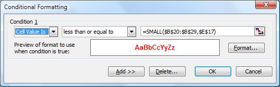
Used with SMALL Function
Highlights lowest nth cells (or whatever # is specified)
Conditional Formatting with the SMALL function is nearly identical. You want Excel to calculate the nth smallest value and then test each value whether is less than or equal to that value. If so, apply the highlighting. Here's what the Conditional Formatting dialog looks like.
Play around with it and once you're confortable with it, it's pretty easy.
Notes
| Last updated | 8/27/08 |
| Application Version | Excel 2003 |
| Author | Michael Kan |
| Pre-requisites |
RANK, LARGE, and SMALL Conditional Formatting: Cell Value Is |
| Related Tips | Conditional Formatting: Formula Is |