
Tips for Excel, Word, PowerPoint and Other Applications
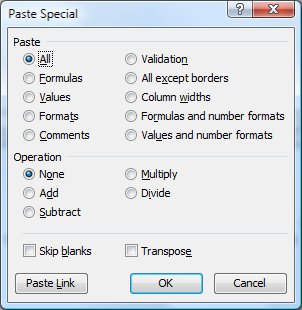
Paste Special (aka ALT + E, S)
Why It Matters To You
Never thought there could be a Tip dedicated to pasting, did you? This is an introduction to a couple of very useful things you can do via the Paste Special (ALT + E, S) function. We'll do a quick overview in this Tip, but it's really a function you need to play around with a bit.
There are many times when we need to either copy calculated data from one worksheet to another without the formulas or transform a data set. This is especially useful when we have columnar data that we want to rotate horizontally for graphic/charting purposes or if we have data that we need to scale up or down by a factor. Paste Special can help out a lot. For anyone up for a challenge, we'll briefly discuss TRANSPOSE at the end of this Tip.
How To ...
You can access Paste Special, after copying a range of cells (Ctrl+C), by either going to the Main Menu, Edit, Paste Special or holding down ALT, then E, S.
When you look at the Paste Special dialog box, you'll see 3 distinct sections, two with radio buttons and 1 with check boxes. As a general rule, you can select combinations of operations limited to 1 radio button per section and any of the check boxes. This will become very apparent once you try out different options.
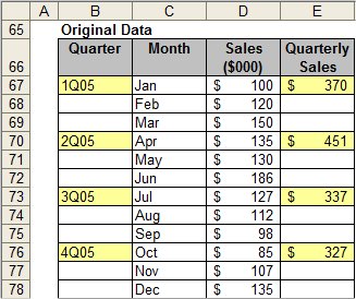
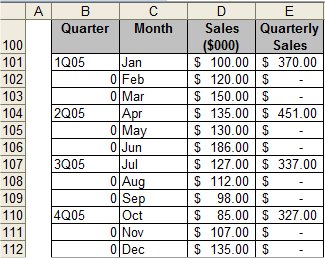
Here's a sample data set I'm going to use for the exercises.
Exercise 1: Paste As Values
One of the most basic application of Paste Special is pasting calculated values as hard coded values. The shortcut you want to use is ALT+Edit (E), Paste Special (S), Values (V) or ALT+E, S, V. Try this out on a couple of cells and take a look at what your end up with after you paste as values. Note that you can do the same thing for Formats, Formulas, or a number of other things.
Exercise 1: Transpose
Let's say I want to make a graph and need my month and sales data to be organized in 2 rows vs. 2 columns. All I need to do is rotate my data, which easily done by the Transpose option in the Paste Special dialog box.
- Select the range C4:D16 then hit CTRL+C to copy the range.
- Activate Paste Special and click on the Transpose check box (the shortcut is ALT + E, S, E)
- Your data should look like this:
- If I only wanted the values, then I could have also clicked the Paste:Values option (ALT + E, S, V, E) which would have returned a result like this:


Exercise 2: Sizing and Scaling
Now I need to convert my 2 column of sales figures into Thousands. I can do this with Paste Special: Operation: Multiply.
How To:
- Add a value anywhere to serve as the multiplier. I'll add a cell with a value of 1000 in G49.
- Select the multiplier then hit CTRL+C to copy
- Highlight the range of numbers you want to transform (C4:D16), then Activate Paste Special: Operations: Multiply (the shortcut is ALT + E, S, M)
- Notice that the transformed data will take on the formatting of your multiplier, so be careful.
- If you did it right, your data should look like the solution set in Column I
- You can use the same set of options to apply a divisor to the entire set, add or subtract an amount to every value.
Exercise 3: Skip Blanks
Let's say that now I need a smaller table, which only shows my quarterly results. Paste Special:Skip Blanks should be able to help me.
How To:
- Hold down CTRL, then click on all of the relevent cells. Holding down CTRL while selecting cells allows you to select multiple, non-contiguous cells. For simplicity, I've shaded in yellow, all of the cells you need to select.
- Hit CTRL+C to copy.
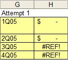
- Select Paste Special:Skip Blanks (the shortcut is ALT + E, S, B)
- Uh oh, what happened? The quarterly sales figures are calculated cells, so we copied the cell fomulas, not the actual values. We'll do this again and also select the column headers.
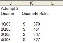
- Select the same cells, but include the column headers
- Hit CTRL+C to copy
- Select Paste Special: Skip Blanks but also select the Values option (the shortcut is ALT + E, S, B, V)
- Your result should look like this:
Exercise 4: Paste Link
From time to time, you may need to replicate data, possibly to another workbook, but link it to your original data Paste Links are useful here, because your linked data will update if the source data ever changes.
Let's use our original data set (C4:D16 for this one.
How To:
- Select the entire range: C4:D16.
- Hit CTRL+C to copy
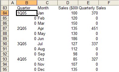
- Select Paste Special: Paste Links (the shortcut is ALT + E, S, L). You'll notice that selecting any other option disables the Paste Links fuction.
- Your result should look like this. Notice that every value is a link back to the corresponding cell in the original table. Try doing this again, but pasting it into a new workbook.
- OK, so we got all of the numbers, but now my formatting is screwed up. That's easy, just select Paste Special: Formats (the shortcut is ALT + E, S, T), and our table is nice and pretty again.
- What you do with the 0 values is up to you. You can leave them as is, or delete them.
Exercise 5: TRANSPOSE, the function
In Exercise 1, we learned how to transpose a pasted range. However, you'll notice that the result are hardcoded values now. What if we want to transpose the links to the original data so that as our analysis changes, the chart data updates accordingly? Here, we want to use the function called 'TRANSPOSE'.
We'll use the data set above. The syntax for the TRANSPOSE function is =TRANSPOSE(array), where the array is the range of cells you want to transpose. In the case of the dataset above, enter, =TRANSPOSE($C$4:$D$16)
Oops, I get a #VALUE! error.
Hmmmm, what happened? TRANSPOSE is an array function, so you have to activate the array. Click on the cell with the TRANSPOSE formula, click on F2 to edit the formula, then hold down CTRL+SHIFT+ENTER. You should see the error value change into 'month'. Now drag and copy the fomula to stretch a full 13 columns x 2 rows, click F2 to edit the formula, then hold down CTRL+SHIFT+ENTER, and the entire range should activate and look like the result below.

For more information on ARRAY operations, take a look at the Introduction to Arrays article
Notes
| Last updated | 8/12/08 |
| Application Version | Excel 2003 |
| Author | Michael Kan |
| Pre-requisites | None |
| Related Tips |
Introduction to Arrays |